1  Get started with R

NoteAbout this edition

This edition introduces the basic ideas behind R and the tidyverse. Some technical explanations and software comparisons are still under review.

R is a programming language designed by statisticians.

Your first goal is to run a saved script, then open a real dataset. This chapter introduces the setup and code you need, then considers where R fits into social-science research: what it asks you to learn and what it makes possible. The final discussion of learning with AI is optional.

Figure 1.1: An example of a ggplot2 figure.

1.1 Downloading R and Positron

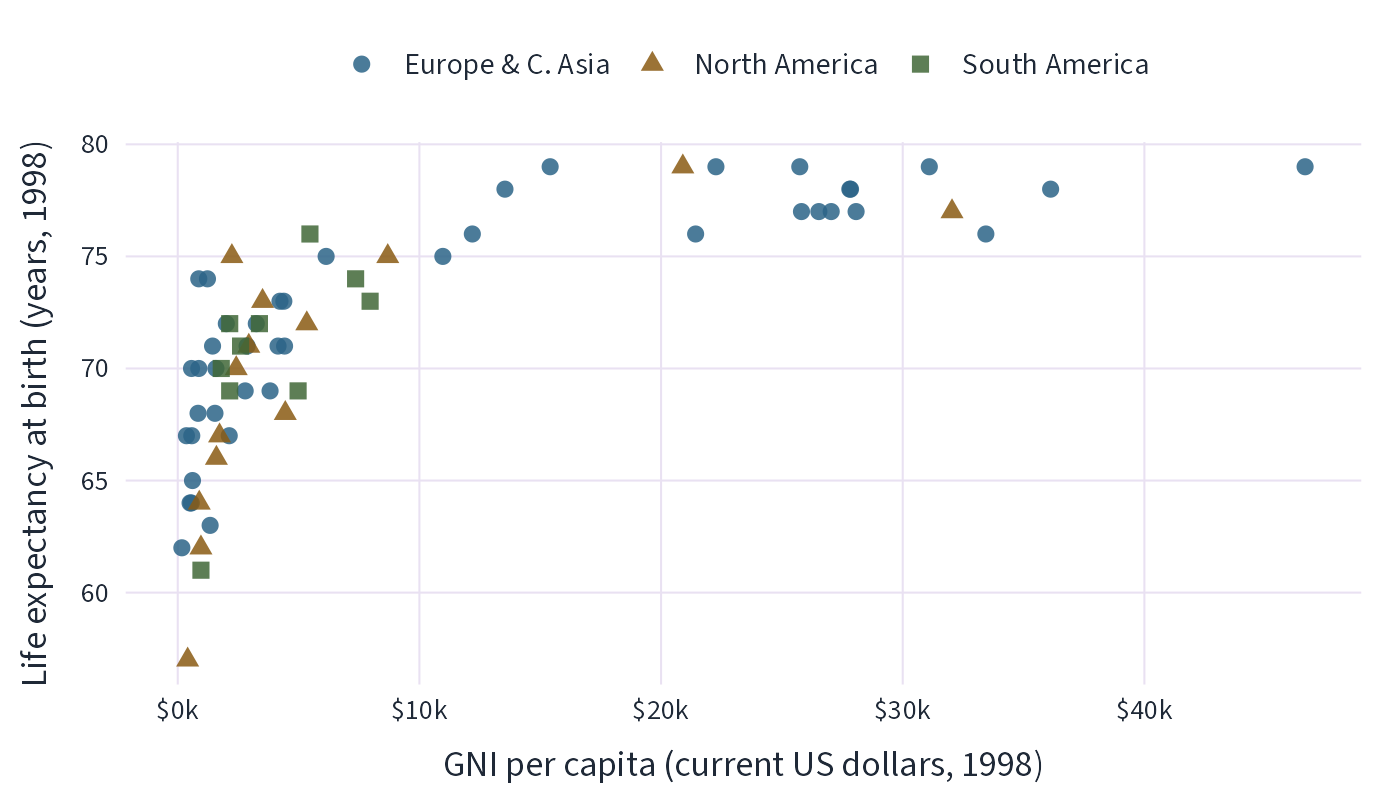
Install two separate programs: R, which runs your code, and an integrated development environment (IDE), which helps you write code, inspect data, and view results. This book uses Positron as its main IDE.

Start by downloading R from the R website. Follow the CRAN link and choose the installer for your operating system. Install R before opening Positron.

Figure 1.2: The R website, with links to download R through CRAN.

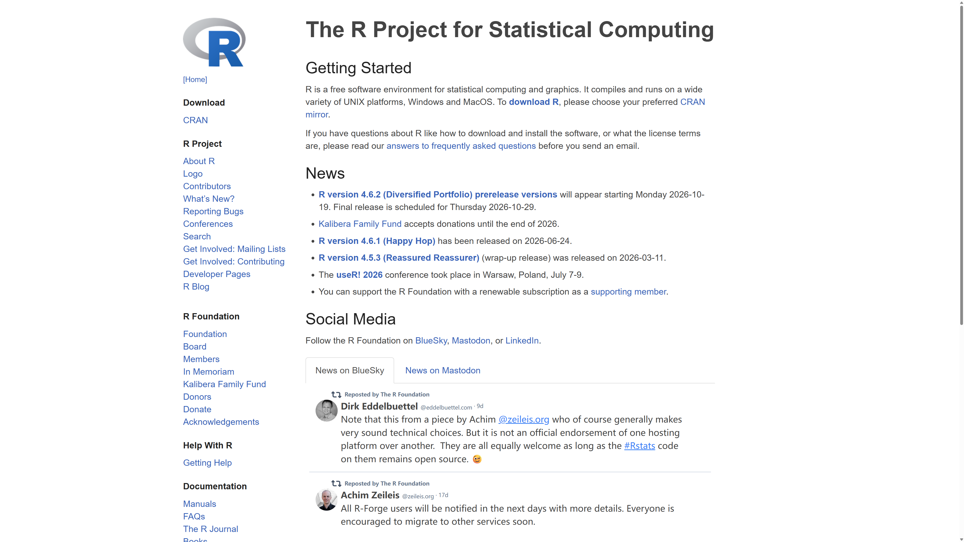
Next, download and install Positron. Choose the installer for your operating system and processor. The website may show a different recommended download on your computer. Positron requires R 4.2 or later; its download page lists any additional system requirements.

Figure 1.3: The Positron download page, shown on Windows.

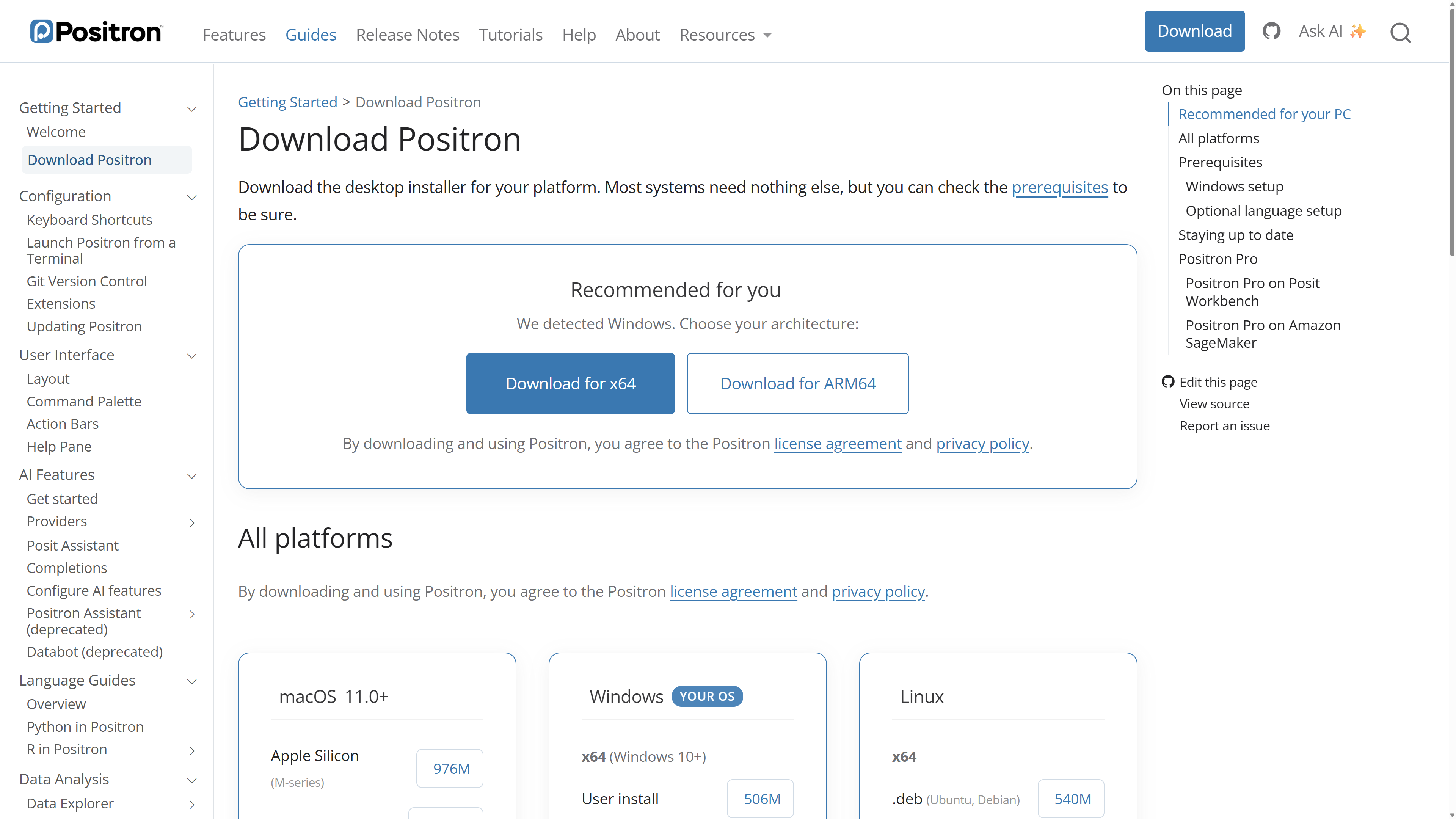
Positron includes support for running R code, exploring data, viewing plots, and reading help. Posit recommends it for new R users. We use one main IDE so that beginners can follow a consistent set of instructions. RStudio remains supported and is a useful alternative if your course already uses it. VS Code also supports R, but its setup requires an R extension and the languageserver package. Readers already comfortable with either editor can continue using it for the R examples in this book.

Figure 1.4: The main regions of Positron, illustrated in Posit’s documentation. Source: Posit Software, PBC.

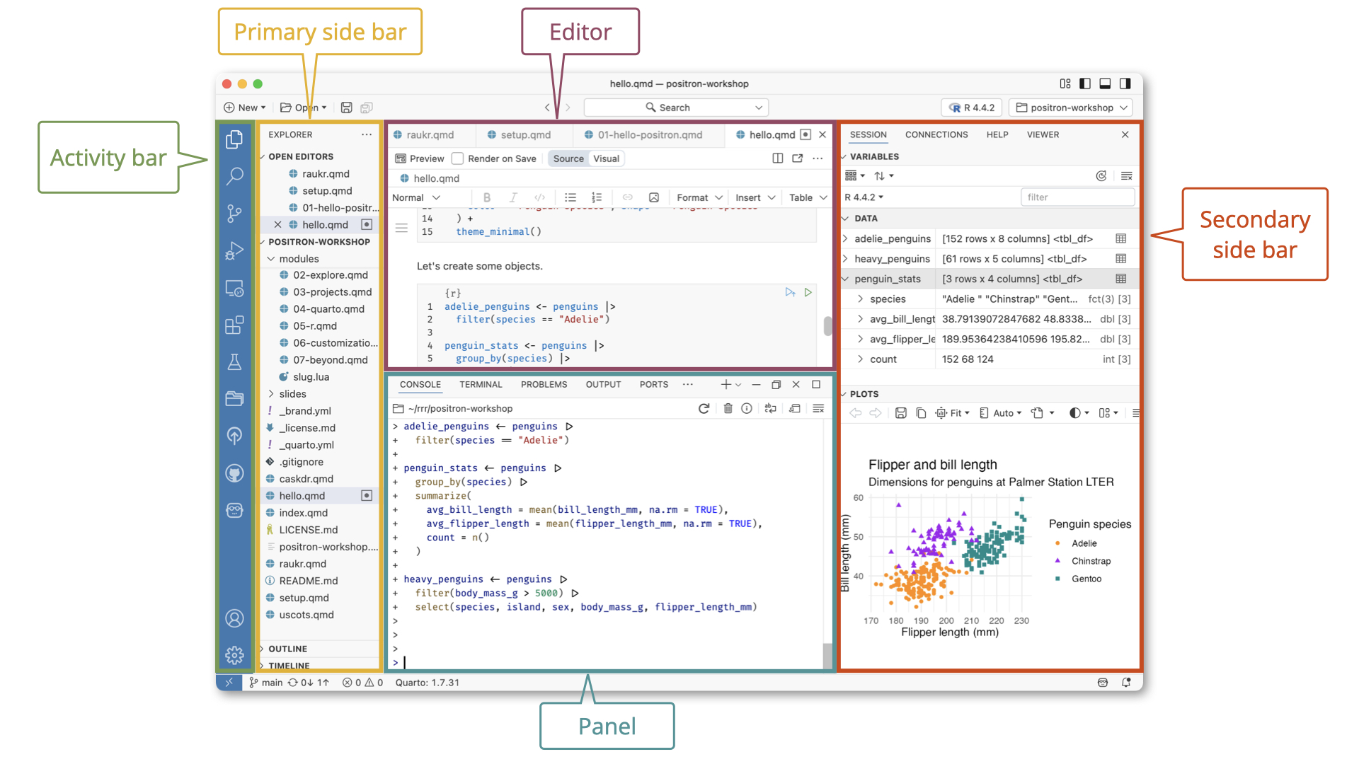
In the layout shown here, the file explorer is on the left, the editor is in the center, and the console is below the editor. The right sidebar contains variables and plots, with tabs for help and other tools. The layout can be customized, so your screen may differ. Open an R script, select an R interpreter if prompted, and use the console to run code. The screenshot is an orientation example from the official documentation; you do not need its example files, packages, or R version.

For now, remember one shortcut: Ctrl + Enter on Windows or Linux, or Cmd + Enter on macOS, runs the selected code in the editor. If no code is selected, Positron runs the current statement.

1.1.1 Keeping your work

Create a folder called r4ss in a location you can find again, such as your Documents folder. Use Positron’s Open Folder command to open it. This is your project folder: keep this book’s scripts, downloaded examples, and saved results together here.

Create a new text file in the editor and save it inside that folder as first.R. The .R extension identifies an R script. Type the examples in the next section into this file, save it, and run statements from top to bottom with the shortcut above. The editor keeps your instructions; the console runs them and displays results. Saving the file keeps the instructions on disk. Running a line creates or changes objects in the current R session.

Reopen this folder and the saved first.R file whenever you resume your work. Saving a script does not preserve the running session’s objects; running its statements in order recreates them. You can also select all the code in a script and run the selection when every line is intended to run. We will check where R reads and writes files when we export our first table in Section 5.5.

1.2 Trying some simple code

Once R and your IDE are installed, we can try a little code. R can perform arithmetic directly:

The shaded R blocks contain code to run; the output appears separately below them. In the console, > is R’s prompt for new input. Do not type that prompt or copy output back as code. An output marker such as [1] identifies the position of the first printed value; it is not part of the answer. Text after # on a code line is a comment for the reader and is ignored by R.

1 + 1

[1] 2

# Make 24 using 3, 4, 5, and 9
(4 + 9 - 5) * 3

[1] 24

In R, quotation marks enclose text:

# Use straight single quotes '' or double quotes "" to represent text
"Hello, R!"

[1] "Hello, R!"

A function performs an operation on supplied inputs and returns a result. Write its name followed by parentheses containing the input. For example, sqrt() takes a number and returns its square root:

# Use sqrt() to calculate a square root
sqrt(25)

[1] 5

The result is 5: five multiplied by itself gives 25. The parentheses make this a function call. The name sqrt refers to the function itself; sqrt(25) calls it on the number 25.

For text, nchar() returns the number of characters. Quotation marks identify the text input:

# Use nchar() to count characters
nchar("hello")

[1] 5

The result is also 5, because hello contains five characters. The two functions perform different operations even though these calls return the same number.

If the console shows + instead of >, R is waiting for the rest of an incomplete expression. For example, typing sqrt(25 leaves its opening parenthesis unmatched:

> sqrt(25
+

The + here is a continuation prompt, not an instruction to add something. Check that parentheses and quotation marks have matching partners. To cancel this unfinished input in Positron, press Ctrl+C with the console focused and no text selected. When the normal prompt returns, enter the complete sqrt(25) again.

For information about a function, enter help("sqrt") in the console. Positron displays its documentation in the Help pane. Find Arguments to see what inputs the function accepts and Examples to see calls you can try. Read the input description before changing a call; help explains the function, while your question determines which input is appropriate.

We can store results for later use:

The arrow <- assigns the result on its right to the name on its left. Assignment is normally silent: a <- 123 stores a value without displaying it. Typing a displays that stored value. a * 2 displays a calculation without changing a, while b <- a * 2 stores that calculation under a second name:

# Assign 123 to a
a <- 123
# Inspect the value of a
a

[1] 123

# Multiply a by 2
a * 2

[1] 246

# Assign the result of a * 2 to b
b <- a * 2
# Inspect the value of b
b

[1] 246

Here, b stores 246. It is a calculated value, not a spreadsheet formula that stays linked to a. If you change a, rerun b <- a * 2 to update b. After restarting R, run a <- 123 before b <- a * 2; running the second line alone in an empty session gives an object-not-found error.

Object names must match exactly, including capital letters: a and A are different names. Creating a does not create A; looking up A gives an object-not-found error unless you have separately assigned it. Prefer short, descriptive lower-case names, with underscores between words, such as income_total. This is a naming convention that helps you read and retype code consistently.

Later chapters deliberately reuse example names such as countries. Running a chapter’s setup replaces an older object with that name in the session. Keep each chapter’s setup with its examples in your saved script, and run the setup before the examples that depend on it.

1.2.1 Values and functions

Store a number under the name x, then display it:

# Store a number
x <- 2.75
x

[1] 2.75

The next line displays the saved value, 2.75. R stores even one number as a vector of length one.

An expression is something R can evaluate to produce a result: a number, a calculation, or a function call. The inputs to a function are called arguments. A comma separates arguments, and = names an argument. round() takes a number and returns a rounded value; its digits argument sets the number of decimal places:

round(x, digits = 1)

[1] 2.8

x

[1] 2.75

The first argument supplies the value and digits = 1 requests one decimal place. The result is 2.8, while x remains 2.75.

Here = supplies an input setting; <- stores a returned result. Later, == will test equality. To keep the rounded result, assign it separately:

rounded_x <- round(x, digits = 1)
rounded_x

[1] 2.8

rounded_x stores 2.8. The original x still holds 2.75.

1.3 Installing R packages

This book mainly uses the tidyverse and tidystata packages. A package adds functions to R. Installing puts a package in a library on your computer; normally you do this once, then install again only when you want an update. Loading with library() makes its functions available in the current session, so repeat that step after restarting R. Installing a package does not load it.

Before continuing, install these two packages. install.packages() downloads from a package repository; pak provides another installer. In pak::pak(), the part before :: names the package and the part after it names the function. This notation calls a function from an installed package without loading the whole package:

# Install tidyverse
install.packages("tidyverse")
# Install the pak installer
install.packages("pak")

Now call pak to install the tested tidystata revision from GitHub:

pak::pak("socimh/tidystata@fd6ef6b9080a7527e870a4bbc5c9c1ff13c7fa46")

These lessons were tested with tidystata 0.4.1 and dplyr 1.2.1. The GitHub revision above fixes the tidystata version used in the examples; installing the current tidyverse supplies dplyr.

When you later run library(tidyverse), attachment messages list the loaded packages. A conflict notice means that two packages supply the same function name; package::function() selects the one you intend. These notices are informational. A message beginning with Error, such as a report that a package is missing, means the requested operation failed and needs attention.

1.4 Data and functions

To understand a line of R code, ask two questions: what data are we supplying, and what do we want to do with them? In the earlier calls, sqrt() received a number and calculated its square root; nchar() received text and counted its characters. Both returned results that we could save with assignment. Data can record information about people, places, and activities; functions let us work with the values representing that information.

Code that contains only data usually does very little. Think of data as nouns and functions as verbs. “Students, scores, average” is a list of words. “Calculate the average of the students’ scores” describes an action. In the same way, a function tells R what to do with data.

NoteNote

In R, data usually act like nouns, while functions usually act like verbs.

1.5 Asking for help

A useful help request lets someone reproduce the problem without your current session. Before sending it:

1. Keep the smallest input and code that still show the problem. Plain values from this chapter are enough for many questions; do not send private respondent records.
2. Include the assignments that create needed objects and any package-loading calls. For round(x, digits = 1), include the preceding x <- 2.75.
3. Copy the exact error message and say what you expected. Here, a successful call should return 2.8.
4. Start a fresh R session and run just the code you intend to share, from the beginning. Check that it reproduces the same problem.

These details help another reader distinguish a missing input, a mistyped name, and an unexpected result.

You have now used functions to calculate results and saved instructions that you can run again. These small examples introduce a way of working that can extend to an entire analysis. Before we open a dataset, consider where that approach is useful and what it requires of you.

1.6 Where R falls short

Writing instructions makes an analysis repeatable, but you must learn the syntax and keep track of the objects those instructions use. In the examples above, running a calculation before creating its input produces an error; changing an input does not automatically update a saved result. Learning to recognize and resolve these problems takes practice.

R also need not replace every tool you already use. If Stata already handles your data, statistical methods, and outputs well, you may have little immediate reason to switch. A useful starting question is whether a recurring research task is becoming difficult to express, repeat, or extend in your current software.

Figure 1.5: Common workflows and the tools often used for them. R is highlighted as this book’s focus.

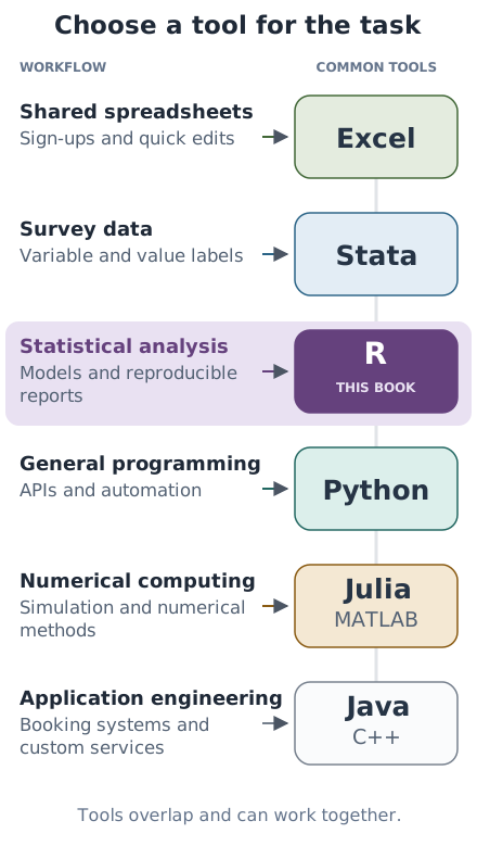
Different tools have their own comfortable areas of use. Stata provides a familiar environment for survey analysis and econometrics. Python is widely used for general programming, web applications, and scientific computing; a project built around a framework such as PyTorch may give you a reason to learn Python. These areas overlap. Choose a language with attention to your research question, collaborators, and the tools you need.

1.7 Where R shines

The same features that take practice can become useful as a project grows. Your saved script already records how to recreate a result, and named objects let you keep inputs and results available together. For many social scientists, the first reasons to develop these habits arise before model fitting. You may need to combine survey files with administrative records, read spreadsheets and data from online services, keep several datasets and intermediate results available, or repeat complicated cleaning across many survey waves. R lets you organize these as named objects and reusable functions. Stata also supports multiple datasets through frames; R’s appeal grows when you want to connect data preparation with a wider range of research tools.

Figure 1.6: Many sources, reusable R code, and different research outputs.

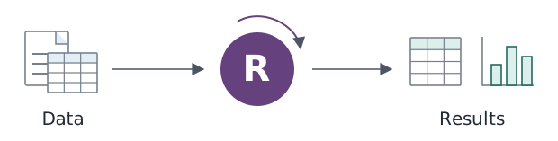
Visualization is another common reason. ggplot2 provides a consistent way to build and refine figures, from a quick check of a distribution to a comparison across groups. The tidyverse connects importing, cleaning, reshaping, and plotting data through related conventions. Learning those conventions can make an entire analysis easier to adapt as your question changes.

See Figure 1.1 for an example of a ggplot2 figure.

As research needs expand, R offers packages for text, spatial, and network data, as well as causal inference, machine learning, simulation, and Bayesian analysis. The CRAN Task Views organize packages by these areas. R can also connect analysis to interactive displays and reports. You can add specialized tools as your work requires them; this book begins with the data preparation, description, and visualization skills that support many such applications.

Some extensions require additional infrastructure. For example, Arrow lets R work with multi-file and larger-than-memory datasets, but installing R alone does not remove memory or computing limits. The value of learning R depends on the workflow it makes possible for you. Its free, open-source ecosystem gives you room to extend that workflow as new needs arise.

We will build on these ideas by comparing ways to organize data in Chapter 2, then choosing columns from a real table in Chapter 3. First, the exercises let you practise calculating with R, storing a value, and using a function. The following discussion of AI is optional; you can go directly to those exercises.

1.8 Learning R with AI [Optional]

You may know what you want to find out before you know the R commands to use. An AI assistant can help you turn that intention into code, explain unfamiliar functions, and get past errors. You can then run the code in R and inspect what it actually does. AI assistance is optional; you can follow this book without it.

1.8.1 Understanding unfamiliar code

Consider five countries from tidystata::lifeexp: Albania, Poland, Canada, Cuba, and Argentina. Their life expectancy at birth is recorded in years. These are rounded World Bank World Development Indicators observations for 1998, distributed with tidystata. We transcribe the five named rows below so that you can inspect every input. The World Bank data are available under CC BY 4.0.

library(tidyverse)

── Attaching core tidyverse packages ──────────────────────── tidyverse 2.0.0 ──
✔ dplyr     1.2.1     ✔ readr     2.2.0
✔ forcats   1.0.1     ✔ stringr   1.6.0
✔ ggplot2   4.0.3     ✔ tibble    3.3.1
✔ lubridate 1.9.5     ✔ tidyr     1.3.2
✔ purrr     1.2.2     
── Conflicts ────────────────────────────────────────── tidyverse_conflicts() ──
✖ dplyr::filter() masks stats::filter()
✖ dplyr::lag()    masks stats::lag()
ℹ Use the conflicted package (<http://conflicted.r-lib.org/>) to force all conflicts to become errors

countries <- tibble(
  country = c("Albania", "Poland", "Canada", "Cuba", "Argentina"),
  lexp = c(74, 73, 79, 75, 73)
)
countries

# A tibble: 5 × 2
  country    lexp
  <chr>     <dbl>
1 Albania      74
2 Poland       73
3 Canada       79
4 Cuba         75
5 Argentina    73

Ask for an explanation. The exchanges here are illustrative; a chatbot or coding assistant may reply differently.

You: Explain this code to a beginner. What does each row represent, and what are the units?

Assistant: library(tidyverse) loads the packages. tibble() creates a table with two columns, country and lexp; c() combines the entries in each column. The arrow <- stores the table as countries. Each row connects a named country with its life expectancy at birth, measured in years.

Typing countries displays the table. Compare Canada’s row with the transcribed code: its recorded value is 79 years. Keeping country names attached to their measurements lets you check which observation an output describes.

1.8.2 From a question to a figure

Describe the result you want. Continue with the same table:

You: Use ggplot2 to compare life expectancy in these five countries in a bar chart. Put countries on the horizontal axis and years on the vertical axis. Explain the code.

Assistant: ggplot() uses the countries table. Inside aes(), country supplies the horizontal positions and lexp supplies the heights. geom_col() draws the bars; labs() sets the axis titles. The + signs add these parts to the plot.

ggplot(countries, aes(x = country, y = lexp)) +
  geom_col() +
  labs(x = "Country", y = "Life expectancy at birth (years)")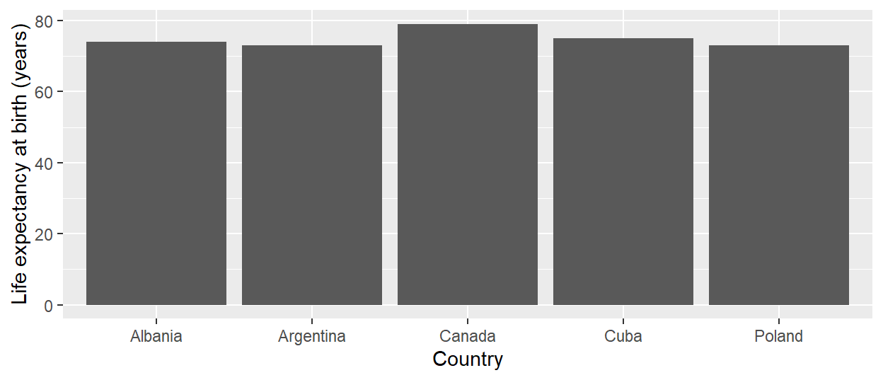

Figure 1.7: Life expectancy at birth in five countries, 1998. Source: World Bank WDI, as distributed in tidystata::lifeexp; rounded years.

Ask about a specific error. If you accidentally type lepx in place of lexp, the plot fails. Include your code and the error when asking for help. Use the help-request checklist in Section 1.5 to make the problem reproducible.

You: My code uses aes(x = country, y = lepx). The error says object 'lepx' not found. The table above has a column called lexp. What is the smallest correction?

Assistant: Change y = lepx to y = lexp. Column names must match exactly.

Run the corrected code and check Canada’s bar against its recorded 79 years. The default display puts country names in alphabetical order, so compare names rather than assuming that the third bar is the third input row. This connects the assistant’s suggestion to a result you can verify.

1.8.3 Checking AI’s suggestions

Check the answer and its meaning. For the same five countries, ask the assistant to calculate the average using dplyr:

summarise(countries, average = mean(lexp))

# A tibble: 1 × 1
  average
    <dbl>
1    74.8

Here, summarise() produces a summary table, mean(lexp) calculates the arithmetic average, and average names the result column. The result is 74.8 years: the five values sum to 374, and 374 divided by 5 is 74.8. Each country contributes equally; this calculation does not weight countries by their population size.

You: Can I conclude that people worldwide had a life expectancy of 74.8 years in 1998?

Assistant: This calculation describes the five selected countries. They were chosen for this teaching example, so their average is not a worldwide estimate. A population-weighted average would also require population counts and a different calculation.

Try the task yourself first. When you need help, ask for a hint or explanation, read the suggested code, predict its result, and run it. AI can help write the commands; knowing the source, units, and selection of observations helps you judge the conclusion.

1.8.4 AI tools [Optional]

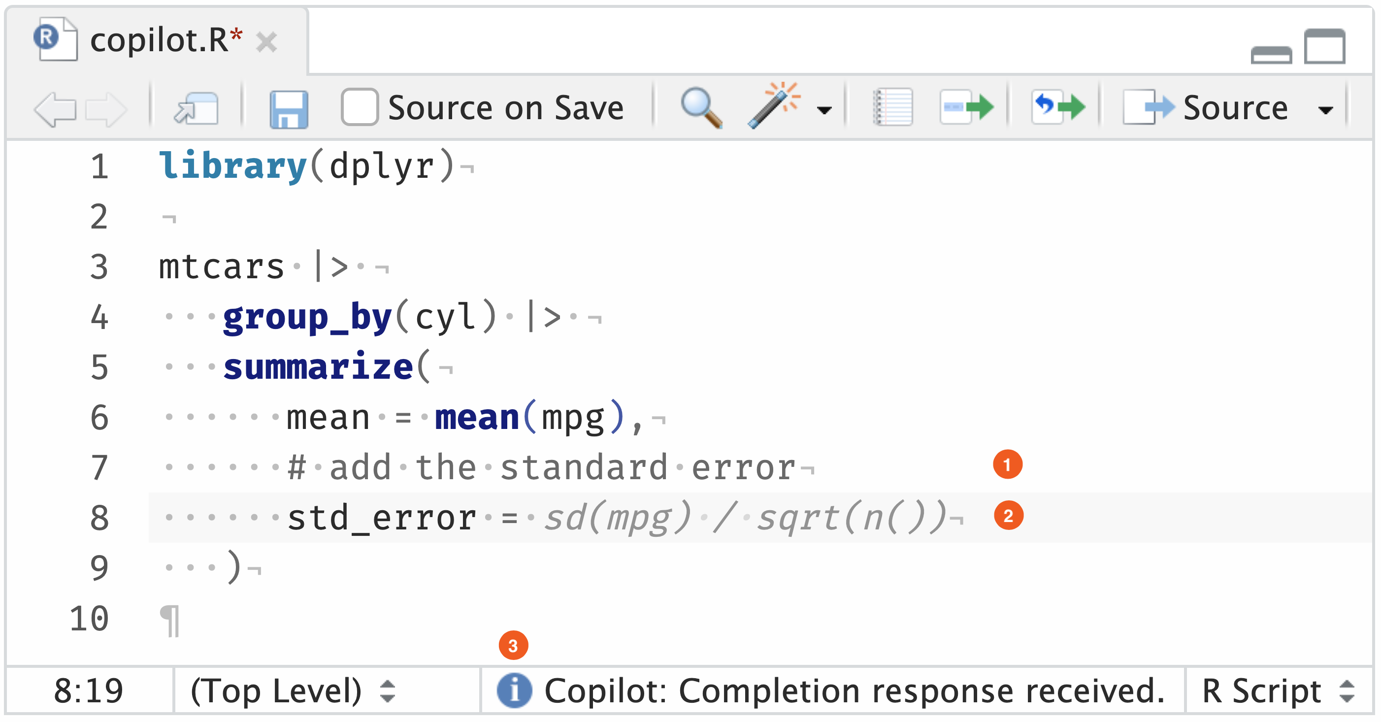
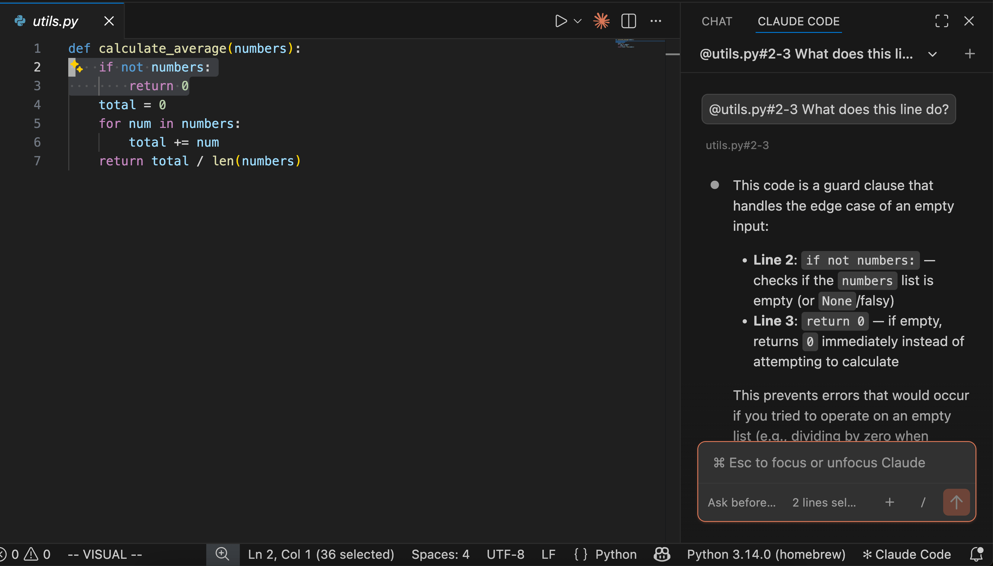
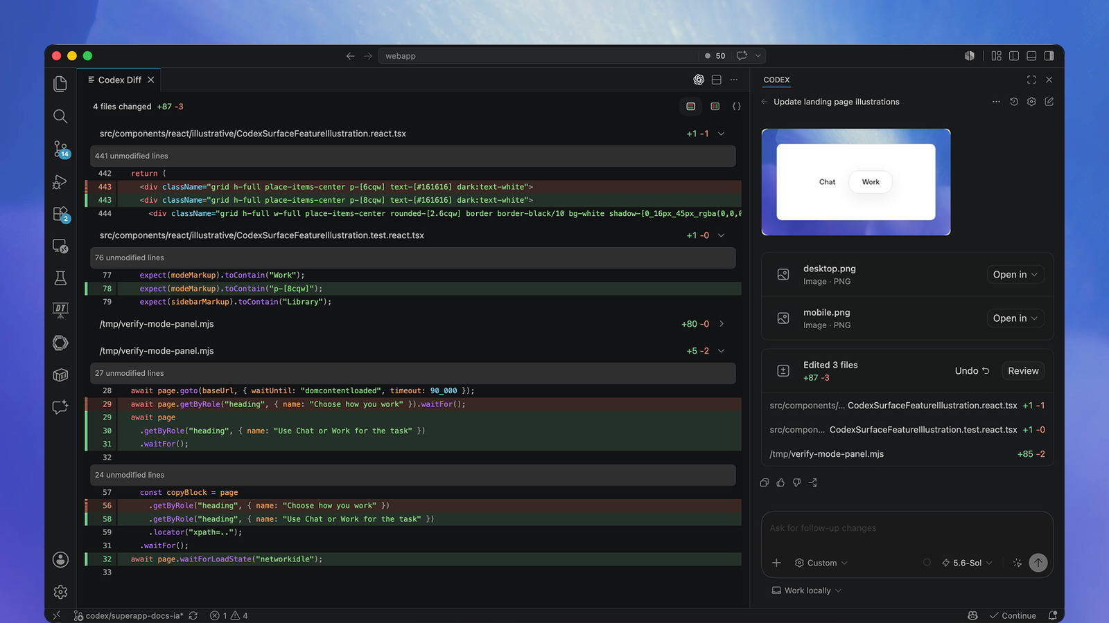
You can ask questions in a chatbot or use an assistant alongside your code. These tools are optional. The tabs show examples from official documentation; their code illustrates the interfaces rather than the country comparison. Select a tab and click its image to enlarge it. Your editor and version may look different.

GitHub Copilot

GitHub Copilot offers code suggestions and chat, depending on the editor. In this RStudio example, a comment describes the task and lighter text shows suggested code. Read a suggestion before accepting it. For our country example, a comment could ask for a ggplot2 bar chart.

Figure 1.8: Copilot suggests code inside RStudio’s editor. Source: Posit Software, PBC, RStudio User Guide.

Claude Code

Claude Code lets you discuss code and request changes. Here, selected code is on the left and a question and explanation appear on the right. You could select the life-expectancy plotting code and ask, “Explain what each line does.”

Figure 1.9: Claude Code explains selected code in VS Code. Source: Anthropic, Claude Code documentation.

OpenAI Codex

OpenAI Codex can work with project files and propose edits. Here, the conversation is on the right and changed lines are visible on the left. You could ask it to fix lepx in the country plotting script, then review the change and rerun the code.

Figure 1.10: Codex presents file changes for review beside its conversation. Source: OpenAI, Codex IDE documentation.

1.9 Review

• <- stores a result under a name; saving a script keeps the instructions for another session.
• sqrt() calculates square roots, nchar() counts characters, and round() rounds numbers.
• help() opens function documentation; include setup, code, and the exact problem when asking for help.
• install.packages() installs packages from CRAN; pak::pak() can install tidystata from GitHub.
• library() loads an installed package for the current session.

Next, Chapter 2 introduces the structures that hold our data and explains why this book mainly uses tibbles.

1.10 Exercises

Practise calculating, saving results, and rebuilding a session from your script. Predict each result before running the code. After trying a question, open the answer with the same number under Worked answers.

1. Calculate with R. In Section 1.2, + adds numbers and * multiplies them. Run these two lines, one at a time. What answer does each line give?

   8 + 2
   8 * 2

2. Saved values and names. Run a <- 10 and b <- a * 2. Predict b after running a <- 12. What must you rerun to update b? Explain why typing A cannot retrieve the value stored as a.

3. Change a function’s input. The function round() rounds a number. Its digits argument tells R how many decimal places to keep, as in Section 1.2.1. Run the line below. Then change digits = 1 to digits = 2 and run it again. What result do you get each time?

   round(2.75, digits = 1)

4. Reconstruct a session. Save these lines in first.R. Restart R with your IDE’s restart command, then run only the last line. Explain the error. Now run the saved script from the beginning and report both values. What did saving the script preserve?

   starting_value <- 10
   doubled_value <- starting_value * 2
   doubled_value

Worked answers

NoteCalculate with R

8 + 2

[1] 10

8 * 2

[1] 16

The first answer is 10: R adds 8 and 2. The second is 16: R multiplies 8 by 2. Changing the symbol changes the calculation.

NoteSaved values and names

a <- 10
b <- a * 2
a <- 12
b

[1] 20

b <- a * 2
b

[1] 24

The first printed b is 20. It stores the earlier calculation; changing a does not recalculate it. Rerunning the assignment to b produces 24. Names are case-sensitive: A is a different name and, unless separately created, gives an object-not-found error. Use the lower-case a to retrieve 12.

NoteChange a function’s input

round(2.75, digits = 1)

[1] 2.8

round(2.75, digits = 2)

[1] 2.75

With digits = 1, the answer is 2.8, rounded to one decimal place. With digits = 2, the answer is 2.75, which already has two decimal places. The number being rounded stays the same; the named argument changes how many decimal places we request.

NoteReconstruct a session

In a fresh session, the last line alone fails because doubled_value has not been created. Run all three saved lines in order:

starting_value <- 10
doubled_value <- starting_value * 2
doubled_value

[1] 20

starting_value

[1] 10

The results are 20 and 10. The script preserved instructions on disk, not the previous session’s objects. Replaying those instructions creates the inputs before they are needed.

Continue to Chapter 2 for a short tour of R objects and a comparison of data-frame and tibble output.